sys.path.append("/home/quant/Documents/Use-Cases")
from engine import Engine
from strategies.rsi2 import RSI2MeanReversion
from strategies.rsi2_final import RSI2MeanReversionFinal
engine = Engine(init_cash=100_000, fees=0.0, fixed_fees=0.0, slippage=0.0000
close = engine.load_data_yf("QQQ", period="max", interval="1d", field="Close
filter_csv = "/mnt/Share8TB/use_cases/Strategy2/Report_2025_10_21__15_39_40/
csv_start, csv_end = engine.apply_prediction_window_from_csv(
csv_path=filter_csv,
prediction_dt_col="PredictionDT",
warmup_days=300,
per_share_fee=0.0035,
)
base = RSI2MeanReversion(
rsi_buy_long=10,
rsi_sell_long=70,
rsi_sell_short=90,
rsi_cover_short=30,
sma_window=200,
)
signals_path_base = "/home/quant/Documents/Use-Cases/signals_csvs/baseline/s
plot_path_base = "/home/quant/Documents/Use-Cases/equity_curves/baseline/equ
os.makedirs(os.path.dirname(signals_path_base), exist_ok=True)
os.makedirs(os.path.dirname(plot_path_base), exist_ok=True)
pf_base = engine.run_backtest(base, export_csv_path=signals_path_base, start
strat_thr = RSI2MeanReversionFinal(
rsi_buy_long=10,
rsi_sell_long=70,
rsi_sell_short=90,
rsi_cover_short=30,
sma_window=200,
prediction_csv_path=filter_csv,
prediction_dt_col="PredictionDT",
score_col="QuantedModelPredictions",
score_threshold=0.6,
force_exit_at_end=True,
)
signals_path_thr = "/home/quant/Documents/Use-Cases/signals_csvs/filtered_co
os.makedirs(os.path.dirname(signals_path_thr), exist_ok=True)
pf_thr = engine.run_backtest(strat_thr, export_csv_path=signals_path_thr)
combined_dir = "/home/quant/Documents/Use-Cases/equity_curves/combined"
os.makedirs(combined_dir, exist_ok=True)
combined_path = os.path.join(combined_dir, "equity_curve_strat2_combined.png
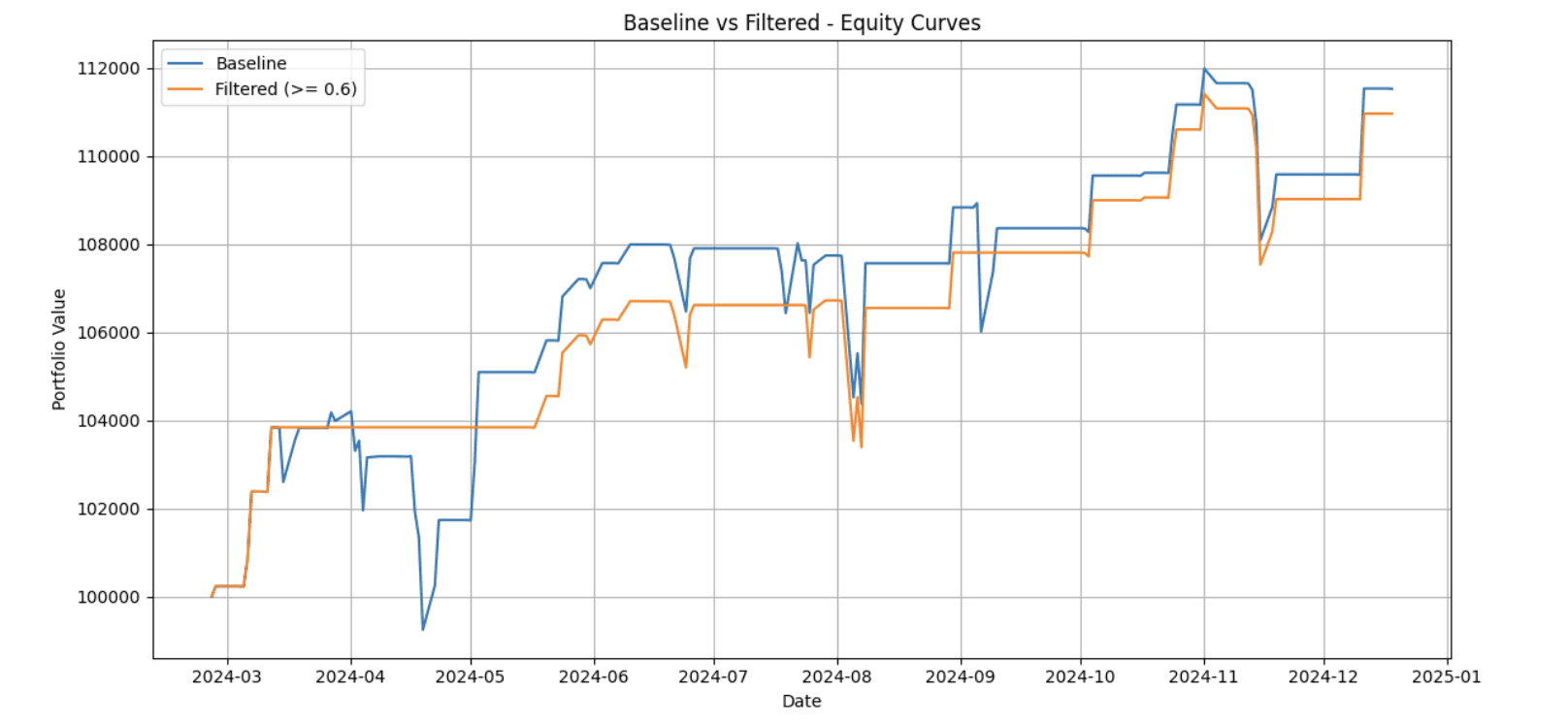
engine.plot_equities(
[
("Baseline", pf_base),
(f"Filtered (>= {strat_thr.score_threshold})", pf_thr),
],
path=combined_path,
show=True,
title="Baseline vs Filtered - Equity Curves",
normalize_to=100000.0,
)
print("Side-by-side Comparison")
stats_base = pf_base.stats()
stats_thr = pf_thr.stats()
thr = getattr(strat_thr, "score_threshold", None)
common = [
"Total Return [%]", "Sharpe Ratio", "Calmar Ratio", "Sortino Ratio",
"Max Drawdown [%]", "Max Drawdown Duration", "Win Rate [%]",
"Total Trades", "Profit Factor"
]
comp = pd.DataFrame({
"Baseline strategy": stats_base.reindex(common),
f"Quanted ML filtered (>= {thr})": stats_thr.reindex(common),
}).round(2)
comp["Δ% (Filtered vs Baseline)"] = (
(comp.iloc[:, 1] - comp.iloc[:, 0]) / comp.iloc[:, 0].replace(0, np.nan)
).round(2)
col_base = "Baseline strategy"
col_filt = f"Quanted ML filtered (>= {thr})"
rows_pct = ["Total Return [%]", "Max Drawdown [%]", "Win Rate [%]"]
rows_num = ["Sharpe Ratio", "Calmar Ratio", "Sortino Ratio", "Total Trades",
row_dur = ["Max Drawdown Duration"]
def fmt_timedelta(v):
if pd.isna(v):
return ""
return f"{(v / pd.Timedelta(days=1)):.2f} days" if isinstance(v, pd.Time
styled = (
comp.style
.format("{:+.2f}%", subset=pd.IndexSlice[:, ["Δ% (Filtered vs Baseli
.format("{:.2f}%", subset=pd.IndexSlice[rows_pct, [col_base, col_fil
.format("{:.2f}", subset=pd.IndexSlice[rows_num, [col_base, col_filt
.format(fmt_timedelta, subset=pd.IndexSlice[row_dur, [col_base, col_
)